


S&P Dow Jones Indices released the July 2026 S&P Cotality Case-Shiller Home Price Index, and the headline will likely receive significant attention: Seattle posted the weakest year-over-year home-price performance among the 20 major metropolitan markets for the second consecutive month.
Seattle home prices were 1.57% below July 2025, while the U.S. National Index increased 1.93%. Seattle’s non-seasonally adjusted index also declined 0.46% from June to July, following a 0.48% decline from May to June.
That headline is real. But it is also important to understand when it happened.
Case-Shiller is telling us about July. We are entering October.
The more useful question for buyers and sellers is: What has happened since then, and what might the fall market be telling us now?
Spring | More Supply Changed the Market
Spring began with increasing inventory and gradually expanding consumer choice. By June, NWMLS-wide active inventory was already 16.4% higher than the prior year, while median prices were 3% lower. Yet transactions had not stopped. June closed sales actually increased 2.3% year over year and 10.2% from May. Buyers and sellers were also dealing with compounding influences from the War in Iran and rising mortgage rates.
The market wasn’t disappearing. It was rebalancing.
More inventory meant buyers no longer needed to make decisions with the same urgency. They could compare homes, evaluate value, and wait for the right opportunity.
For sellers, that meant the return of something we hadn’t experienced to the same degree during the low-inventory years: competition. Accurately pricing this market was becoming more critical.
Summer | From Scarcity to Selectivity
By July and August, the consequences became more apparent.
The new S&P report confirms that Seattle prices declined during June and July (and it will repeat in August). National prices were still appreciating, but Seattle was experiencing a regional correction. S&P describes a continuing East-West divergence, with Seattle registering the lowest annual return among the 20 cities it follows.
Buyers became more selective. Decision cycles lengthened. Price reductions became more common. Inspection, financing, and other contingencies returned to negotiations. Homes that were differentiated, well-presented, and priced to meet the market could transact, while overpriced properties increasingly competed for a smaller pool of buyers.
The August statistics reinforce that experience. Across NWMLS, active inventory was 22% higher year over year, while closed sales were 7.6% lower and median prices were 2.3% lower. Months of inventory increased from 3.19 a year earlier to 4.21 months.
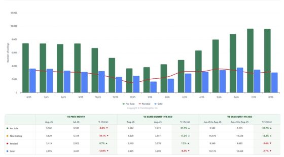
And within our primary King, Snohomish, Pierce, and Kitsap County resale market (matching the S&P data set), the Trendgraphix data we’ve been reviewing make the supply/demand divergence even more pronounced:
August 2026 vs. August 2025:
- For Sale: 9,582 — +31.7%
- New Listings: 4,629 — +17.2%
- Pending Sales: 3,119 — +1.3%
- Closed Sales: 2,995 — –9.2%
That is the summer 2026 story in four numbers: inventory expanded dramatically faster than absorption.
Fall | Watch the Rate of Change
Now comes the interesting part. Our Trendgraphix “Today’s Stats” through September 27 don’t yet indicate a broad sales acceleration. But they do suggest the market may be entering a different phase.
Active inventory remains extremely elevated at 9,696 homes, +31.3% year over year. But September new listings are only +1.3% year over year—a dramatic moderation from August’s +17.2%.
Meanwhile, September pending sales are just 1.3% below last year, while closed sales remain 11.9% lower.
That distinction matters; perhaps buyers are encouraged by improved selection and sharper pricing with room to negotiate, and worries about mortgage rates rising further? Remember, you can always “re-fi”, but you can’t “re-buy,” so the strike price matters more than the interest rate.
Closings tell us where the market was. Pending sales provide a better indication of where transactions may be heading.
September’s 2,368 closings largely represent purchase decisions made during the softer late-summer environment. September’s 2,623 pending contracts are more contemporary evidence of buyer behavior.
So, while it would be premature to declare a fall recovery, there are early signs that the rate of deterioration may be moderating.
See the following supply/demand illustration for the subject area through August 2026 below:
Meet the Market
This fall is unlikely to reward aspirational pricing simply because a seller remembers what a neighbor achieved in another market cycle.
With roughly 31% more active inventory than a year ago across our four-county dataset, every listing is competing against a substantially larger peer group.
For sellers, the relevant question is no longer simply:
“What did the last home sell for?”
It is:
“What else can today’s buyer purchase for the same money?”
Identify what makes your property unique and highlight those features to interested buyers.
A listing that starts behind the market can accumulate days on market, chase subsequent price reductions, and ultimately reinforce a buyer’s perception that something is wrong. A compelling property appropriately positioned against its current competition has a much better opportunity to capture the buyers who are active now.
For buyers, this is a very different market from the inventory-constrained environment of recent years.
There is more selection. There can be more negotiating leverage. Sellers may be more receptive to contingencies and thoughtful terms.
But desirable properties that are correctly priced can still attract competition.
The objective isn’t to “time the bottom.” It is to recognize value when today’s combination of property, price, terms, and personal circumstances makes sense.
To discuss the data and your real estate goals with a market expert, reach out to a Global Real Estate Advisor.